Neural networks for quantum many-body physics

17 Jun 2024 in Blog

A quick intro to the neural networks for quantum many-body physics. Basic quantum background encouraged but not necessary.

---

There is no doubt - AI has seen some tremendous advances in the past decade.

Just to mention a few examples:

• Large language models surpassed human performance¹ on a multitude of tasks,
• AlphaZero humbles the world’s top chess players,
• AlphaFold2&3 make a huge impact on protein folding research.

This impressive progress across diverse disciplines naturally leads me to wonder about my own field:

Can recent AI advancements aid in understanding quantum many-body physics?

In my view, the answer is a qualified yes! Why? Well, maybe because neural networks are already state-of-the-art for some quantum many-body physics models among all existing numerical methods! Neural networks for many-body problems are highly-expressible, efficient and have a different set of limitations than existing numerical methods. Cool! This suggests a potentially interesting space of problems where neural networks might outperform traditional methods. Motivated by this why not learn more about neural networks for quantum?

In this blogpost I will discuss how to apply neural-network based methods for solving quantum many-body problems. We will start by briefly describing the basic framework. This should give enough background to understand the current literature on the topic. Equipped with this knowledge, we will talk about the hopes and rather unique strengths of neural networks for some quantum problems as compared with other existing methods. These will include the lack of an inherent sign problem (as compared with quantum Monte Carlo) and not being limited to area law entanglement states (as compared with tensor networks). Finally, we will discuss some associated challenges and provide an outlook of this emerging field.

Within the blogpost, I will assume you have some quantum background. I recognize though that this is an interdisciplinary field, so to make things a bit clearer for machine-learning-inclined people, please read through the extra expandable “ML boxes” to get a bit more of the quantum context. Alright, let’s get started!

• Neural networks for quantum - basics
  • Representating a quantum state
  • Sampling quantum ground state energy
  • Energy optimization
• Neural networks for quantum - hopes
  • Expressivity of neural networks for quantum
  • Efficiency and ML community
  • No sign problem
• Neural quantum states: challenges
  • Local minima issue and ground states
  • Challenges for time dynamics
• Outlook
• FAQ
• References
• Hints to exercises

Neural networks for quantum - basics

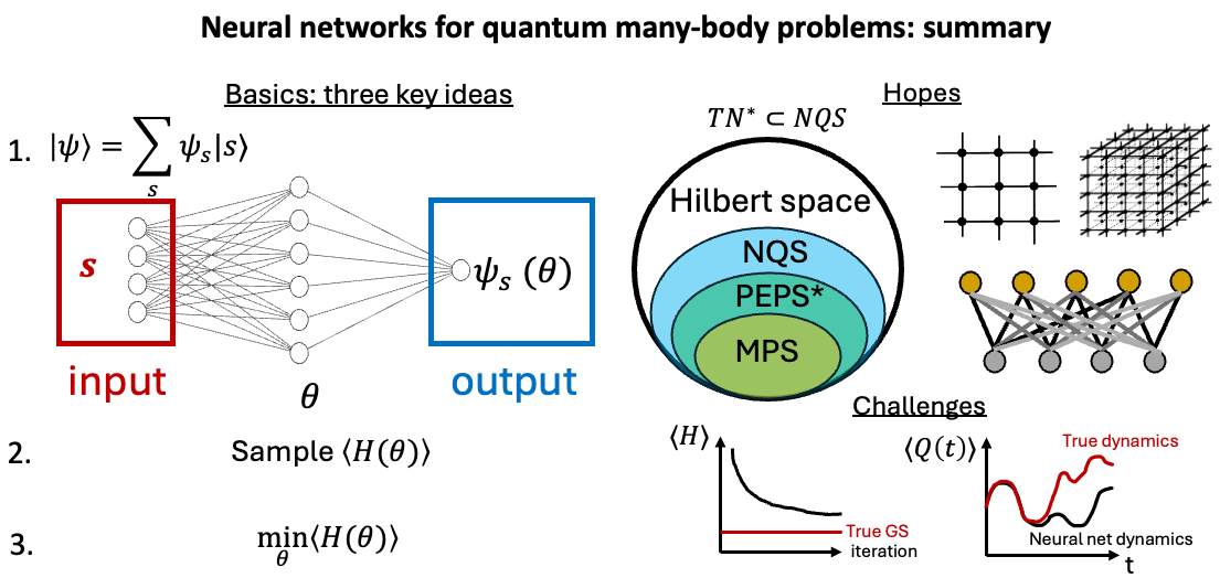
We will study the problem of finding the lowest energy states or time dynamics of a quantum many-body system. The basics of applying neural networks to it are really simple. We will consider three key ideas [Carleo&Troyer (2017)]:

1. Expand a quantum state in a certain basis where coefficients will be parametrized by a neural network.
2. Treat an expectation value of a Hamiltonian as a loss function and evaluate it through sampling.
3. Optimize the loss function by the steepest descent on neural network parameters.

Note, all this is purely optimization: there is no data and we utilize neural networks only as (powerful!) function approximators². For simplicity, we will focus on spin Hamiltonian models, but the formalism below extends to fermions and bosons as well.

Representating a quantum state

ML BOX 1: Notation, quantum states and inner products.

In quantum mechanics, the state of a system, such as a collection of “qubits” (spins \(1/2\)) is represented as a vector \(|\psi \rangle\) in a tensor product Hilbert space. For a system with \(N\) qubits, this Hilbert space has a dimension \(2^N\). Any vector in this space might be decomposed in a complete basis of length \(N\) combinations of 0’s and 1’s. For instance \(|000\rangle = |0\rangle \otimes |0\rangle \otimes |0\rangle\) for \(N=3\) corresponds to a basis vector \(e_0=(1,0,0,0,0,0,0,0)\). To denote vectors in a Hilbert space \(\mathcal{H}\) physicists often use bra-ket notation where “ket” is denoted by \(|\psi \rangle \in \mathcal{H}\) and dual vector “bra” by \(\langle \phi | \in \mathcal{H}^{*}\). In such notation, an inner product becomes \(\langle \phi | \psi \rangle \in \mathcal{C}\). A quantum mechanical expectation value of an operator \(Q\) in state \(|\psi \rangle\) then can be written as \(\langle \psi | Q \psi \rangle\). Throughout we assume working with an orthonormal basis \(\langle i|j\rangle = \delta_{ij}\) thus e.g., \(\langle 000 | 001 \rangle = \langle 0 | 0 \rangle \langle 0 | 0 \rangle \langle 0 | 1 \rangle = 0\). If you feel uncomfortable with using bra-ket notation just think of \(|\psi \rangle\) as a \(2^N\) dimensional complex vector \(\psi\) (decomposable into an orthonormal complete basis as \(\psi = \sum_i \psi_i e_i\) where \(e_i^{\dagger} e_j = \delta_{ij}\)), inner product \(\langle \phi | \psi \rangle\) as \(\phi^{\dagger} \psi\) where \({\dagger}\) denotes conjugate transpose, and \(\langle \psi | Q \psi \rangle\) as a quadratic form \(\psi^{\dagger} Q \psi\).

Let’s begin by writing a many-body quantum state on \(N\) qubits and expand it in a complete, orthonormal basis: \begin{equation} |\psi \rangle = \sum_{s} \psi_s |s \rangle \end{equation} where \(\{|s\rangle\}\) are basis vectors (e.g., in a computational basis \(|s\rangle=|100\rangle\) for \(N=3\)) and there will be \(2^N\) bit string elements. The key point now is to parameterize complex coefficients \(\psi_s\) as a neural network \(\psi_s (\theta)\) where \(\theta\) is a vector of all neural network parameters. Such a neural network takes as an input a bit string (e.g., \(s=\{-1,1,1\}\) corresponding to the example above) and outputs a complex number \(\psi_s\) - see the figure below.

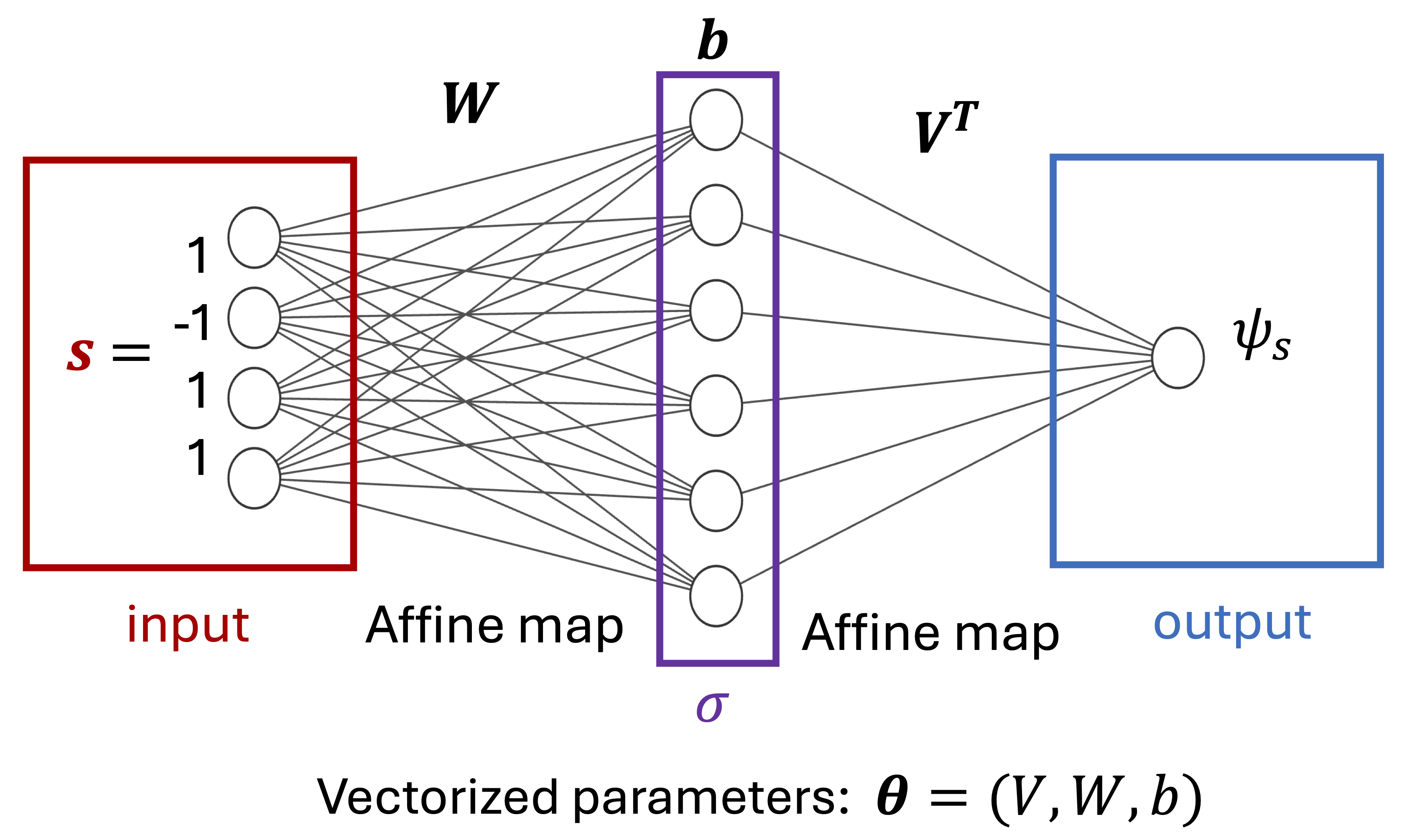
Fig. 1: A simple example of a neural network for a quantum many-body problem. \(W \in \mathbb{C}^{N_{hidden}\times N}\), \(V^T \in \mathbb{C}^{1 \times N_{hidden}}\) are trainable matrices, \(b \in \mathbb{C}^{N_{hidden}}\) is a trainable (bias) vector and \(\sigma(x)\) denotes a non-linearity e.g., RELU.

Neural network parameterizes the wavefunction of a quantum system in a particular way i.e. represents it as a series of affine transformations interspersed by non-linear (activation) functions for each input bit string. For instance, for the architecture above we have \(\psi_s = V^T σ(Ws+b)\) and \(\theta= (V,W,b)\).

Key idea 1: Decompose a many-body quantum state \(|\psi \rangle= \sum_{s} \psi_s |s \rangle \) and represent \(\psi_s (\theta)\) coefficients as a neural network with parameters \(\theta\).

Sampling quantum ground state energy

Okay, so far we have parameterized wavefunctions with a neural network. But how do we solve different classes of many-body problems with this approach? Perhaps conceptually simplest class of problems in this context is finding the lowest-energy (ground) states of a Hamiltonian which we will dive into next. Solving other classes of problems, like time dynamics or steady states in open systems, follows a similar logic, and we will touch on those later.

ML BOX 2: What is a "ground state" and why search for it?

In a quantum many-body physics problem of \(N\) qubits we are typically given a \(2^N \times 2^N\) (Hamiltonian) matrix \(H\). It turns out that a lot of the interesting low-temperature behavior of such a system might be captured by studying the lowest-eigenvalue eigenvector (“ground state”) of the Hamiltonian matrix. The exact approach (known as exact diagonalization) would be to numerically diagonalize the Hamiltonian matrix, however, due to its exponential size (in \(N\)) it becomes quickly infeasible as \(N\) grows beyond 20’ish qubits. This is why approximate methods for finding such eigenvectors are needed (most well-established ones largely fall into “tensor network” and “quantum Monte Carlo” camps). One paradigm for approximately finding ground states is using the variational principle which states that \begin{equation} \min_{\theta} \frac{\psi^{\dagger} (\theta) H \psi (\theta)}{\psi^{\dagger} \psi} \geq \lambda_{min} \end{equation} where \(\lambda_{min}\) is the lowest-lying eigenvalue of \(H\). Therefore utilizing a parametrized ansatz for a quantum state \(\psi(\theta)\) we can find an approximation to the lowest-lying eigenvalue (and correspondingly to the lowest-lying eigenvector) by optimizing over parameters \(\theta\). In this blogpost, we intend to parametrize this variational ansatz with a neural network and then treat \(\frac{\psi^{\dagger} (\theta) H \psi (\theta)}{\psi^{\dagger} \psi}\) as a loss function.

Consider a quantum system governed by a Hamiltonian \(H\). We will variationally approach the problem of finding a ground state of this Hamiltonian. In other words, we will try to minimize an energy: \(\langle H (\theta) \rangle\) with respect to the parameters of a neural network \(\theta\). Let’s be a little more explicit about this: \begin{equation} \min_{\theta} \langle H \rangle = \min_{\theta} \frac{\psi^{\dagger} (\theta) H \psi (\theta)}{\psi^{\dagger} \psi} \end{equation}

To proceed let’s expand the above formula in an orthonormal basis (dropping \(\theta\) for conciseness):

\begin{equation} \langle H \rangle = \frac{\sum_{s} \sum_{s’} \psi_{s}^{\ast} \langle s | H |s’ \rangle \psi_{s’}}{ \sum_r \sum_q \psi_r^{\ast} \psi_q \langle r | q \rangle} = \frac{\sum_{s} \sum_{s’} \psi_s^{\ast} H_{s s’} \psi_{s’}}{ \sum_r |\psi_r|^2} \end{equation} where \(H_{s s'} = \langle s | H |s' \rangle\) are matrix elements of a Hamiltonian \(H\).

To further proceed let’s assume³ that \(\psi_s \neq 0\), we can divide and multiply by \(\psi_s\) to get \begin{equation} \langle H \rangle = \sum_s p_s E_{loc}(s) \end{equation} where \(p_s = \frac{|\psi_s|^2}{\sum_{s'} |\psi_{s'}|^2}\) is a probability mass function over bit strings and \(E_{loc}(s) = \sum_{s'} H_{s s'} \frac{\psi_{s'}}{\psi_s}\).

Exercise: Convince yourself that the above derivation is correct by filling-in the missing steps by yourself!

Now, here comes the key practical question: can we compute \(E_{loc}(s)\) and \(\langle H \rangle\) efficiently? Note that what we have done above is mostly rewriting of the original exponentially-hard problem and, indeed, both quantities in principle involve sum over all bit string elements - and there are still \(2^N\) of them…

Let’s consider \(E_{loc}(s)\) first. Although, for a fully generic Hamiltonian matrix will be dense, Hamiltonians corresponding to typical physical systems will be quite sparse! In particular, for a given bit string \(s\) (row of an exponentially large Hamiltonian matrix), there will be only polynomially many (in \(N\)) non-zero entries. This implies that summation over \(s'\) in \(E_{loc}(s)\) might be performed efficiently.

Exercise: Consider a simple form of an Ising model \(H_{ising}=\sum_{i=0}^{N-1} X_i X_{i+1}\) in 1D with periodic boundary conditions. Convince yourself that there will be only \(\mathcal{O}(N)\) non-zero entries per bit string element Hint.

That is great, but how about \(\langle H \rangle\) evaluation? Well, utilizing the form of \(\langle H \rangle\) we derived above, our best strategy is to evaluate a sum over exponentially many elements through sampling: \begin{equation} \langle H \rangle \approx \frac{1}{N_{samples}} \sum_{i=1}^{N_{samples}} E_{loc}(s_i) \end{equation} where set of samples \(\{s_i\}\) are typically generated by a Metropolis-Hastings algorithm⁴ and \(\{s_i\}\) make a Monte Carlo Markov Chain (MCMC).

At first, it might sound a bit wild! In MCMC we create a chain of bit string configurations used for sampling \(s_0 \rightarrow s_1 \rightarrow \cdots \rightarrow s_{N_{samples}}\). If the update rule is ergodic⁵ then the MCMC chain will eventually converge to sampling from an underlying true probability distribution. However, the required chain length (or mixing time) can be uncertain and sometimes exponentially long for some adversarial examples of distributions. So why doesn’t it ruin the method above? Here are a few practical reasons for this:

1. For ground states of stoquastic Hamiltonians, the MCMC chain is provably polynomial in system size [Bravyi+ (2023)]⁶.
2. One can just ‘hope for the best’ and monitor some quality characteristics of MCMC methods (such as autocorrelation timeand Rsplit) which can often detect sampling issues.
3. For specific neural network architectures, such as autoregressive networks, MCMC methods are not needed - one can use more reliable direct sampling [Sharir+ (2019)].

Key idea 2: Estimate expectation value of energy (loss function) through Monte Carlo Markov chain sampling.

Energy optimization

Great! So we know how to evaluate energy efficiently, but how to minimize it? The answer is simple: steepest descent!

In the simplest form, it will correspond to a gradient descent algorithm for neural network parameters \(\theta\) \begin{equation} \theta_{t+1} = \theta_{t} - \eta \nabla_{\theta} \langle H \rangle \end{equation} where \(\eta\) denotes learning rate. Note that the above gradient descent might be thought of as stochastic gradient descent (SGD) since we evaluate gradients \(\nabla_{\theta} \langle H \rangle\) by sampling (as discussed before).

So why do I say the steepest descent instead of just SGD? Well, in practice, standard SGD often falls short in accuracy for most architectures and models. More advanced optimization methods such as quantum natural gradient [Stokes+ (2020)] (in the quantum Monte Carlo community also known as stochastic reconfiguration [Sorella (1998)]) are usually required. The main idea of these methods is to take into account “curvature” information of the underlying parameter space manifold and therefore perform an update in a “steeper” direction than that proposed by a gradient itself. Typically such extra information is hidden in a (stochastic approximation of) matrix \(\mathbf{S}_{\alpha, \beta} = \mathbb{E} \left[ \left( \frac{\partial \log \psi_{s}(\theta)}{\partial \theta_{\alpha}} \right)^{*} \left( \frac{\partial \log \psi_{s}(\theta)}{\partial \theta_{\beta}} \right) \right] - \mathbb{E} \left[ \left( \frac{\partial \log \psi_{s}(\theta)}{\partial \theta_{\alpha}} \right)^{*} \right] \mathbb{E} \left[ \frac{\partial \log \psi_{s}(\theta)}{\partial \theta_{\beta}} \right]\) with dimensions \(N_{parameters} \times N_{parameters}\) (often known as quantum geometric tensor) which is said to precondition the usual gradient i.e. a quantum natural gradient update is defined by \begin{equation} \theta_{t+1} = \theta_{t} - \eta \mathbf{S}^{-1} \nabla_{\theta} \langle H \rangle \end{equation} where \(\mathbf{S}^{-1}\) denotes (pseudo)inverse of an \(\mathbf{S}\) matrix. Although I will postpone discussing \(\mathbf{S}\) matrix (which is quite an interesting object!) in more detail for another blogpost, here are three key practical points:

1. Quantum natural gradient is essentially performing quantum imaginary time evolution on a variational manifold [Stokes+ (2020), Appendix B],
2. Quantum natural gradient updates are more costly⁷ than standard SGD. They require calculating matrix (pseudo)inverse, increasing computation complexity to \(\mathcal{O}(N_{parameters}^3 + N_{parameters}^2 N_{samples})\) or after information re-packaging \(\mathcal{O}(N_{samples}^3 + N_{parameters} N_{samples}^2)\), see [Chen&Heyl (2023)],
3. Matrix \(\mathbf{S}\) is ill-conditioned and therefore needs regularization before it can be inverted. This is usually done by adding a small diagonal shift, \(\mathbf{S} \rightarrow \mathbf{S} + \epsilon \mathbb{I}\), to improve the condition number.

We will revisit the quantum geometric tensor \(\mathbf{S}\) in more detail when we get to challenges section!

Key idea 3: Optimize the expectation value of energy through (stochastic) steepest descent.

Neural networks for quantum - hopes

Wonderful! So far we have studied three key ideas for applying neural networks to quantum many-body problems (often known as neural quantum states). To recap:

1. Represent the coefficients of a quantum state using a neural network,
2. Sample the expectation value of energy to get the loss function⁸,
3. Optimize this loss function through the steepest descent methods.

Very simple! But why is this approach helpful? Long story short: expressivity, efficiency inherited from the ML community and no sign problem (in principle) are keywords. Let’s explore these in more detail!

Expressivity of neural networks for quantum

Let’s start with expressivity. We aim to approximate a quantum state in a Hilbert space \(\psi \in \mathcal{H}\) with a parametrized ansatz \(\psi(\theta)\). One cool thing about neural network ansatze⁹ is their ability to capture any state in a Hilbert space, given that the network is wide enough. More specifically, even a single hidden layer neural network can approximate any quantum state with arbitrary precision, as the number of neurons in the hidden layer goes to infinity (see Fig. 2 below).

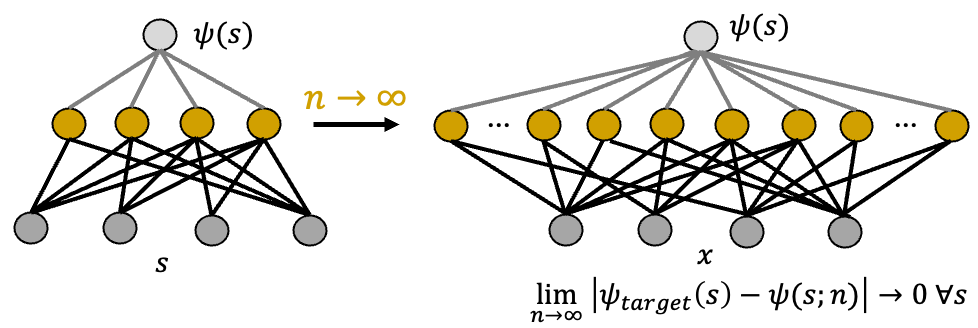
Fig. 2: A simple sketch of a universal approximation theorem.

ML BOX 3: Tensor networks and area law, quantum Monte Carlo and sign problem.

Tensor network and quantum Monte Carlo methods have been used in condensed matter/quantum many-body physics for over 20 years.

Tensor Networks

In tensor network methods (see this review), each coefficient in a quantum state basis expansion is treated as a tensor with N indices. The most common form, Matrix Product States (MPS), decomposes a large tensor with \(2^N\) numbers into a network of tensors with \(\mathcal{O}(N \chi^2)\) parameters, where \(\chi\) is the bond dimension.

• The catch is that the above representation is practical only if \(\chi \sim \mathcal{O}(\text{poly} N)\), which applies to quantum states following the "area law" of entanglement. This means von Neumann entanglement entropy across any system boundary scales with the "area" of that boundary.In 1D, the boundary is a point, so entropy is constant. In 2D, the boundary is a line, scaling entropy with system size. In 3D, entropy grows with the boundary, corresponding to an "area." States with faster-growing entanglement (e.g., "volume" law) make tensor networks impractical as \(\chi\) scales exponentially with \(N\).
• Evaluating observables in a tensor network requires "contracting" the network (summing over indices). This is efficient for MPS, however, for systems of larger dimensionality (2D, 3D etc.) better-suited tensor network formulations, such as project entangled pair-states (PEPS) are not always efficiently contractible (which again limits their use).

Quantum Monte Carlo (QMC)

QMC methods (see this book) evaluate multi-dimensional integrals arising in descriptions of a many-body problem (e.g., a path integral, partition function etc.).

• QMC is not limited by system dimensionality, handles finite temperature systems, and scales well to large systems.
• However, QMC faces the "sign problem," requiring exponentially many samples for accurate integrals. This is commonly the case in fermionic or non-stoquastic Hamiltonians, making QMC impractical for these cases.

Above is a cute theoretical limit but it does not sound terribly practical: \(N_{parameters} \rightarrow \infty\) guarantee is even worse than \(2^N\) coefficients required to naively represent any quantum state… But here comes a nice result: suppose one restricts to \(N_{parameters} \sim \mathcal{O}(poly(N))\). How much of a Hilbert space can one still cover? Well, [Sharir+ (2020)] proved that it is strictly more than efficiently contractible¹⁰ tensor networks: see Fig. 3 below.

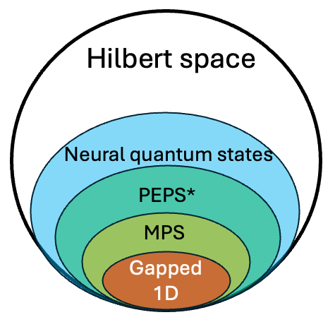
Fig. 3: Expressivity of different many-body ansatze if one restricts to polynomially many parameters [Sharir+ (2020)].

In particular, unlike tensor networks, there exists volume law states [Deng+ (2017)] which may be represented by simple neural network architectures (such as restricted Boltzmann machines) with only a polynomial number of parameters. This makes neural networks, in principle, hopeful for representing ground states of some long-range interacting Hamiltonians or quantum states arising from long quench dynamics! What is the rough intuition behind the efficient representability of the volume law?

Short answer: non-locality of connections within hidden units of the neural network (which contrasts with local connectivity of tensor networks). For instance, [Deng+ (2017)] proves that for a simple example of a restricted Boltzmann machine architecture¹¹, restricting connections between the input layer and a hidden layer to \(\mathcal{O}(1)\) neighbors upper bounds representable entanglement entropy to an area law. On the other hand, they prove that there exist examples of RBM states (with a polynomial number of parameters) with long-range (\(\mathcal{O}(N)\)) connections which exhibit volume law - see Fig. 4 below. Thus, it is long-range connectivity which allows for efficient description of some volume law states¹².

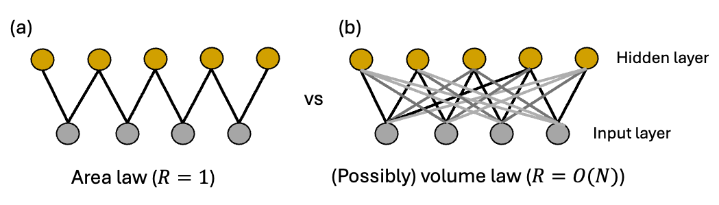
Fig. 4: Volume-law in restricted Boltzmann machines requires long-range connectivity.

This is cool: neural quantum states are strictly more expressive than tensor networks, and their representability is limited by something different than entanglement thus making it applicable to cases where tensor networks fall short! But then a natural question becomes: what physical quantity limits neural network expressivity on quantum states? I.e. what is an equivalent of “entanglement” for tensor networks or “magic” for efficient quantum circuit simulation? Well, as of mid-2024, we do not yet have a clear answer and this remains a thrilling open problem!

Hope 1: Neural quantum states are strictly more expressive than (efficiently contractible) tensor networks.

Efficiency and ML community

The expressivity of neural quantum states is nice, but it is not enough. We need to not only know that a solution exists but also be able to find it efficiently! And here comes another good thing about neural networks: thanks to extensive machine learning research and commercial incentives, neural quantum states (if deployed right!) benefit from a lot of efficiency of running ML models¹³. What does it mean in practice? It allows to access finite-size numerics on large system sizes, also in 2D, 3D and beyond!¹⁴ This is again unlike tensor networks, which although can tackle 2D or even 3D systems, might potentially suffer from (i) contraction issues and (ii) memory and runtime issues¹⁵. These capabilities were demonstrated by finding state-of-the-art ground states of e.g., 40x40 square lattice Rydberg Hamiltonian [Sprague&Czischek (2024)] or a transverse field Ising model on a 21x21 square lattice [Sharir+ (2019)].

Hope 2: Neural quantum states are "quite" efficient both runtime and memory-wise.

No sign problem

Accessing large system sizes in reasonable times on lattices in 2D and 3D is not unique to neural networks: in many cases, methods such as quantum Monte Carlo can also achieve this. But here comes another advantage of neural quantum states: they can tackle sign-problem-full Hamiltonians where quantum Monte Carlo is typically hopeless. For instance, [Chen&Heyl (2023)] achieved state-of-the-art results on sign-problem-full spin J1-J2 Heisenberg model, and others successfuly studied (sign-problem-full) fermionic systems (see e.g., [Moreno+ (2022)]).

Is the sign problem fully gone though? Well, there is no free lunch¹⁶. Achieving accurate energies on sign-problem-full Hamiltonians with neural quantum states is typically more challenging than in a sign-problem-free case [Szabo&Castelnovo (2020)]. The difficulty might be tracked further to an appropriate representation of the phase structure of the quantum states¹⁷. Although, some progress has been made in this direction by using a greater number of parameters [Chen&Heyl (2023)], bridging tensor networks with neural networks [Chen+ (2023)], or pre-training on data from quantum simulators / other numerical methods [Lange+ (2024)], properly dealing with involved phase structure of quantum wavefunctions remains an important open problem.

Hope 3: Neural quantum states do not suffer from a sign problem (at least in principle!).

Neural quantum states: challenges

Okay, we have seen plenty of qualified hopes for neural quantum states. What are the key extra challenges?

Local minima issue and ground states

Well, for ground states of more complicated Hamiltonians, optimization often gets stuck in local minima (see Fig. 5).

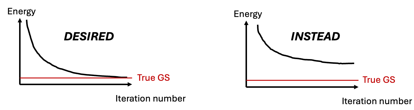
Fig. 5: Neural network optimization often gets stuck in local minima.

Unfortunately, this is often true even as one ramps up the number of parameters in a neural network. This is not good as it leaves us without a clear way to systematically improve solution accuracy. Recent work [Dash+ (2024)] links such “practical breakdown” of scalability to properties of a quantum geometric tensor i.e. matrix \(\mathbf{S}\) we mentioned in the optimization section: saturation of accuracy scalability corresponds to a saturation in the rank of the quantum geometric tensor.

Practically, however, optimization getting trapped in local minima remains an important problem. One hopeful direction is incorporating symmetries for neural networks. In traditional machine learning community this problem is quite well studied and comes under umbrella term of “equivariant machine learning” (or even wider, geometric deep learning), and was shown to be one of the key building blocks for one of the most successful neural networks models to date, such as AlphaFold2&3. In the neural quantum states community, enforcing symmetries has been also studied and shown to improve the quality of local minima by orders of magnitude (see for instance [Vieijra+ (2020)] for an \(SU(2)\) symmetry, or [Roth+ (2020)] for inclusion of lattice symmetries). The key intuition is that the larger the symmetry group, the greater the benefit, as it effectively reduces the accessible Hilbert space.

Interestingly, as we demonstrate in our recent work [Kufel+ (2024)] it turns out that the physical symmetries do not need to be “perfect” and inclusion of only approximate symmetries for neural networks can lead to comparable, orders of magnitude improvements in accuracy over unbiased neural network architectures¹⁸!

Challenge 1: Ground state search with neural quantum states is often stymied by getting trapped in local minima.

Challenges for time dynamics

Okay, enough of problems for ground states! Let’s briefly touch upon time dynamics.

First a little background. It turns out, that finding the time-evolution of quantum states might be found in a very similar neural quantum states paradigm which we described before. We still represent wavefunction with a neural net, sample observables, and optimize with the quantum natural gradient (although with a slightly modified loss function). As it turns out, due to the close connection with imaginary time evolution, the only small change for real-time dynamics is a modified loss function that introduces an extra imaginary unit \(i\) in front of the natural gradient updates.

This approach of simulating time-dynamics with neural quantum states already has seen some successes e.g., in achieving state-of-the-art (in some regimes) for simulating parameter sweep through a \(20 \times 20\) square lattice transverse field Ising model [Schmitt+ (2022)]. Unfortunately, more broadly, time evolution with neural quantum states seems to be a more challenging problem than finding ground states. This manifests itself in e.g., inaccurate long-time observable evolution trajectories (see Fig. 6).

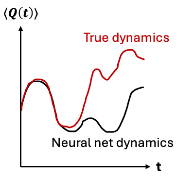
Fig. 6: Neural networks often struggle to capture long-term dynamics of an observable \(Q\).

To an extent such worse behavior is to be expected: time dynamics is more challenging for tensor networks as well! Here are some neural-network-specific reasons that complicate the accurate simulation of real time dynamics:

1. Necessity of complex phases in simulating dynamics leading to similar issues discussed in the no-sign-problem section,
2. Regularization required for ill-conditioning of quantum geometric tensor \(\mathbf{S}\) (see the optimization section) can divert the ansatz away from the true physical trajectory¹⁹,
3. Stochastic estimation of \(\mathbf{S}\) matrix is crucial for time-dynamics, and its Monte Carlo estimations are prone to biased sampling issue. This relates back to assuming \(\psi_s \neq 0 \ \forall s\) we have made in derivation of Monte Carlo estimates before: it turns out whenever \(\psi_s \approx 0\) while \(\partial_{\theta} \psi_s \neq 0\), Monte Carlo estimates of \(\mathbf{S}\) will be biased, rendering accurate real-time dynamics tracking to be more difficult [Sinibaldi+ (2023)].

Despite these challenges, in my view, improving time dynamics with neural quantum remains a promising open research direction, with some exciting applications such as benchmarking quantum simulators (see e.g., [Shaw+ (2024)])!

Challenge 2: Time dynamics with neural quantum states requires careful handling of sampling and regularization.

Outlook

I hope I have convinced you that neural networks for quantum many-body physics might be a promising research direction. We have explored how to solve many-body problems variationally by using neural networks to represent wavefunction coefficients, sampling energy and optimizing with respect to the network parameters. We highlighted the advantages of this approach, including strictly greater expressibility than (efficiently contractible) tensor networks, efficiency in memory and runtime and the ability to handle sign-problem-full Hamiltonians. We also discussed the challenges of neural quantum states which for ground states corresponded to ansatze getting trapped in local minima. This is quite a bit of stuff - congratulations on staying with me until this point.

Of course, we have only scratched the surface of neural network methods for quantum many-body physics! If you would like to learn more about them see the FAQ section below with further reading suggestions and stay tuned for future blogposts on related topics!

FAQ

1. What are typical neural network architectures used for quantum many-body physics problems? Initially restricted Boltzmann machines and fully-connected networks were popular. As of 2024, architectures incorporating symmetries, like convolutional neural networks or more broadly group-convolutional neural networks, have shown a lot of success. Furthermore, recently, autoregressive neural networks (such as recurrent neural networks or transformers) have also become promising due to their ability to produce independent samples, improving Monte Carlo estimates of observables. See [Lange+ 2024(b)] for a nice, recent, review.
2. What other classes of quantum many-body physics problems were studied with AI methods? Oh boy, there is a lot! One example is studying steady states of open quantum systems (see e.g., [Nagy&Savona 2019] ). Another example, much closer to a supervised learning setup is quantum state tomography i.e. figuring out what is a quantum state (or what values observables defined on such quantum state take) given a set of experimental measurement snapshots. For more details see e.g., [Torlai+ (2018)] review or more recent provable advantages of ML methods for state tomography [Huang+ (2022)]. Neural quantum states may be also applied to continuous molecular systems, fermionic or bosonic models and quantum circuit simulation. For a short review on this see [Medvidović&Moreno (2024)]. For a more comprehensive, broader overview, check this older review or this book on ML for quantum physics. Finally, note that throughout this blogpost we have talked about simulating many-body physics on classical computers. A field of Quantum machine learning is concerned with running (ML) algorithms on quantum computers - which is quite a bit different to what we discussed above!
3. I am interested in experimenting with neural quantum states, how do I start? Try NetKet, a cool open-access neural network library for quantum many-body physics in Python. With extensive tutorials in its documentation and integration with advanced ML libraries like JaX, you will start smoothly with neural quantum states!

Acknowledgements: I thank Jack Kemp, DinhDuy Vu, Chris Laumann and Norm Yao for many fun discussions on neural quantum states and beyond. I also thank Shashvat Shukla and Arthur Pesah for their helpful comments on the draft of this blogpost. Feel free to contact me at dkufel (at) g.harvard.edu if you have any questions or comments!

References

Arjovsky+ (2015) Arjovsky, M., Shah, A. and Bengio, Y., 2016, June. Unitary evolution recurrent neural networks. In International conference on machine learning (pp. 1120-1128). PMLR.

Bravyi (2023) Bravyi, S., Carleo, G., Gosset, D. and Liu, Y., 2023. A rapidly mixing Markov chain from any gapped quantum many-body system. Quantum, 7, p.1173.

Carleo&Troyer (2017) Carleo, G. and Troyer, M., 2017. Solving the quantum many-body problem with artificial neural networks. Science, 355(6325), pp.602-606.

Chen&Heyl (2023) Chen, A. and Heyl, M., 2023. Efficient optimization of deep neural quantum states toward machine precision. arXiv preprint arXiv:2302.01941.

Chen+ (2023) Chen, Z., Newhouse, L., Chen, E., Luo, D. and Soljacic, M., 2023. Antn: Bridging autoregressive neural networks and tensor networks for quantum many-body simulation. Advances in Neural Information Processing Systems, 36, pp.450-476.

Dash+ (2024) Dash, S., Vicentini, F., Ferrero, M. and Georges, A., 2024. Efficiency of neural quantum states in light of the quantum geometric tensor. arXiv preprint arXiv:2402.01565.

Deng (2017) Deng, D.L., Li, X. and Das Sarma, S., 2017. Quantum entanglement in neural network states. Physical Review X, 7(2), p.021021.

Huang+ (2022) Huang, H.Y., Kueng, R., Torlai, G., Albert, V.V. and Preskill, J., 2022. Provably efficient machine learning for quantum many-body problems. Science, 377(6613), p.eabk3333.

Kufel+ (2024) Kufel, D.S., Kemp, J., Linsel, S.M., Laumann, C.R. and Yao, N.Y., 2024. Approximately-symmetric neural networks for quantum spin liquids. arXiv preprint arXiv:2405.17541.

Lange+ (2024) Lange, H., Bornet, G., Emperauger, G., Chen, C., Lahaye, T., Kienle, S., Browaeys, A. and Bohrdt, A., 2024. Transformer neural networks and quantum simulators: a hybrid approach for simulating strongly correlated systems. arXiv preprint arXiv:2406.00091.

Lange+ (2024)(b) Lange, H., Van de Walle, A., Abedinnia, A. and Bohrdt, A., 2024. From Architectures to Applications: A Review of Neural Quantum States. arXiv preprint arXiv:2402.09402.

Medvidović&Moreno (2024) Medvidović, M. and Moreno, J.R., 2024. Neural-network quantum states for many-body physics. arXiv prep

Moreno+ (2022) Robledo Moreno, J., Carleo, G., Georges, A. and Stokes, J., 2022. Fermionic wave functions from neural-network constrained hidden states. Proceedings of the National Academy of Sciences, 119(32), p.e2122059119.

Nagy&Savona (2019) Nagy, A. and Savona, V., 2019. Variational quantum Monte Carlo method with a neural-network ansatz for open quantum systems. Physical review letters, 122(25), p.250501.

Roth+ (2023) Roth, C., Szabó, A. and MacDonald, A.H., 2023. High-accuracy variational Monte Carlo for frustrated magnets with deep neural networks. Physical Review B, 108(5), p.054410.

Schmitt+ (2022) Schmitt, M., Rams, M.M., Dziarmaga, J., Heyl, M. and Zurek, W.H., 2022. Quantum phase transition dynamics in the two-dimensional transverse-field Ising model. Science Advances, 8(37), p.eabl6850.

Sharir+ (2019) Sharir, O., Levine, Y., Wies, N., Carleo, G. and Shashua, A., 2020. Deep autoregressive models for the efficient variational simulation of many-body quantum systems. Physical review letters, 124(2), p.020503.

Sharir+ (2019b) Levine, Y., Sharir, O., Cohen, N. and Shashua, A., 2019. Quantum entanglement in deep learning architectures. Physical review letters, 122(6), p.065301.

Sharir+ (2022) Sharir, O., Shashua, A. and Carleo, G., 2022. Neural tensor contractions and the expressive power of deep neural quantum states. Physical Review B, 106(20), p.205136.

Shaw+ (2024) Shaw, A.L., Chen, Z., Choi, J., Mark, D.K., Scholl, P., Finkelstein, R., Elben, A., Choi, S. and Endres, M., 2024. Benchmarking highly entangled states on a 60-atom analogue quantum simulator. Nature, 628(8006), pp.71-77.

Sorella (1998) Sorella, S., 1998. Green function Monte Carlo with stochastic reconfiguration. Physical review letters, 80(20), p.4558.

Sprague&Czischek (2024) Sprague, K. and Czischek, S., 2024. Variational Monte Carlo with large patched transformers. Communications Physics, 7(1), p.90.

Stokes+ (2020) Stokes, J., Izaac, J., Killoran, N. and Carleo, G., 2020. Quantum natural gradient. Quantum, 4, p.269.

Szabo&Castelnovo (2020) Szabó, A. and Castelnovo, C., 2020. Neural network wave functions and the sign problem. Physical Review Research, 2(3), p.033075.

Torlai+ (2018) Torlai, G., Mazzola, G., Carrasquilla, J., Troyer, M., Melko, R. and Carleo, G., 2018. Neural-network quantum state tomography. Nature Physics, 14(5), pp.447-450.

Vieijra+ (2020) Vieijra, T., Casert, C., Nys, J., De Neve, W., Haegeman, J., Ryckebusch, J. and Verstraete, F., 2020. Restricted Boltzmann machines for quantum states with non-Abelian or anyonic symmetries. Physical review letters, 124(9), p.097201.

Hints to exercises

Hint: Consider e.g., \(N=4\) and \(\vert 0000 \rangle\) bit string. How many \(\langle s' \vert\) exist such that \(\langle s'\vert H_{ising} \vert 0000 \rangle \neq 0\)?

1. See e.g., this for evaluating the GPT-4 and GPT-3.5 for ophthalmology self-assessment program. ↩︎

2. This is one of the key differences between neural networks for quantum setup and typical supervised learning: we do not need to worry about generalization, only about minimizing the loss function as much as possible. ↩︎

3. You might ask why is it valid to make this assumption? Well, in general, it is not and for some problems, this assumption is violated and introduces a bias to the sampling method! It will be further discussed here. ↩︎

4. In case you are unfamiliar with Metropolis-Hastings algorithm: the key idea is to (i) start from a random bit string \(s_0\) (ii) generate another bit string \(s_1\) by applying an update rule to \(s_0\) (e.g., flip a bit at a random location), (iii) calculate acceptance probability for \(s_1\) (for symmetric update rules as in the example above: \(\min(1,\frac{\vert \psi_{s_1} \vert^{2}}{\vert \psi_{s_0} \vert^{2}})\)) and (iv) draw a number uniformly from range \([0,1]\), if it is below or equal to the acceptance probability calculated in (iii) then accept, if not then reject the \(s_1\) configuration and draw a new bit string (v) repeat to construct a Monte Carlo Markov chain. ↩︎

5. Ergodic in our case means that such an update rule allows us to explore all bit string space. ↩︎

6. To completely rule out sampling inefficiency for stoquastic Hamiltonians, one might need to potentially show that sampling is efficient throughout the entire optimization path. This means that starting with initial parameters \(\theta_{0}\) and converging to the ground state parameters \(\theta_*\) sampling might need to be provably efficient not just at \(\theta_0\) but also for all intermediate states between \(\theta_0\) and \(\theta_*\). However, it is not immediately clear to me if efficient sampling at every point along the path is truly necessary! ↩︎

7. Such increased computational cost is prohibitive for models with a huge number of parameters and thus the classical counterpart of a quantum natural gradient is rather rarely used in practice in classical machine learning! ↩︎

8. In practice, step 2 and step 3 would be done together when e.g., using automatic differentiation. ↩︎

9. Note that this is not true for generic variational ansatze! ↩︎

10. Just a reminder: evaluating observables on tensor networks such as MPS or PEPS requires contracting a tensor network. Although efficiently contracting MPS is always efficient, contracting PEPS is in general a #P-complete problem (think exponentially hard). The efficient contractibility requirement is helpful for the expressivity proof in the linked reference (efficiently contractible tensor networks are mapped to neural networks that perform efficient contractions). ↩︎

11. You may roughly think of restricted Boltzmann machines as a feed-forward 1 hidden layer neural network architecture with \(\log \cosh\) non-linearites and product aggregation in the final layer. ↩︎

12. Another, more direct, intuition comes from studies of convolutional neural networks (or more specifically so-called “convolutional arithmetic circuit) by [Sharir+ (2019b)]. These operate based on sliding kernels of size \(K \times K\) (in 2D) each time moving by stride of size \(S\), applying non-linearities and repeating this operation in \(L\) layers. It turns out that for 2D systems the maximum amount of entanglement of a subsystem of size \(\alpha \times \alpha\) as represented by the above neural network with stride \(S=1\) is lower bounded by \(L K \alpha\). This implies that as long as \(L K > \alpha\), such neural network architecture can support volume law entanglement (only with \(L K^2\) parameters)! Authors point out that the key component which allows for efficient representation of volume law comes from information re-using when subsequent kernel moves overlap (e.g., tree tensor network would correspond to \(S=K\) which corresponds to non-overlapping kernels). Fun fact: handwavingly this condition might be turned upside down and applied to classical ML in an interesting recent paper [Alexander+ (2023)]: successful application of using locally connected neural networks (such as convolutional neural networks with \(\mathcal{O}(1)\) size kernels) requires quantum entanglement of the underlying data to be “small”! ↩︎

13. By this I mean a few things: first existence of efficient libraries benefiting from automatic differentiation, vectorization and just-in-time compilation (such as JAX) and second existence of hardware tailored for collecting multiple passes through a neural network in parallel such as GPUs or TPUs. ↩︎

14. In 1D application of neural networks does not make so much sense since matrix product state methods just work incredibly well! ↩︎

15. DMRG algorithm has an unfavorable \(\mathcal{O}(N \chi^3)\) runtime complexity (where \(\chi\) is a bond dimension). ↩︎

16. This seems like more of a general pattern: recent results suggest that computational difficulty of tensor network contraction to an extent also suffers from a sign-problem. ↩︎

17. Note that the presence of complex phases in the outputs of the neural networks is another difference between neural quantum state and more traditional machine learning setup. Although there are some works e.g., [Arjovsky+ (2015)] in such setup and operate on complex parameters, they point out that the performance of these models sensitively depends on the choice of non-linearities for complex numbers. Alternatively, one can work with real parameters and create two networks: one learning a real phase \(\phi\) and the other a real amplitude \(A\) (only later combining them by \(A e^{i \phi}\)), but this approach has also seen only a limited success [Szabo&Castelnovo (2020)] ↩︎

18. Approximate symmetries naturally appear in the context of Hamiltonians perturbed away from the symmetric fixed points, typical of experimental setups! An interesting example is the celebrated class of quantum spin liquid Hamiltonians which exhibits an exponentially large group of approximate symmetries in their ground states. See our paper for more details! ↩︎

19. Although the presence of regularization decreases the accuracy of the neural quantum states for ground state search as well, it is much less of an issue there. The reason is that \(\epsilon\) regularization parameter(see optimization section for definition), interpolates between quantum natural gradient (aka imaginary time evolution) and “standard” gradient update. Therefore even in \(\epsilon \rightarrow \infty\) limit, such optimization is admissibile for ground states (simply ignoring curvature information). This contrasts with time dynamics problems where no such limit exists. ↩︎