2D toric code - intro to a loopy subject without going in circles

13 May 2023 in Blog

A real quick introduction to the 2D toric code viewed from the condensed matter angle. No background other than basic quantum mechanics required.

Working in the field of quantum technologies I often chat to people from a variety of quantum-focused fields. A weird thing happens if people from traditionally different communities talk about the same stuff. This is how I first heard about the toric code: both condensed matter and quantum error correction people spoke about it a lot. Soon afterwards I discovered why: toric code is a paradigmatic example for both topological quantum error correction and topological order in condensed matter. What makes this model to be famous and which of its properties make it so fun to work with?

In this blogpost, I would like to answer these questions by discussing the toric code basics as viewed from the perspective of condensed matter physics: for a complimentary viewpoint from the quantum error correction perspective see excellent post by Arthur Pesah. In section 1 we will discuss the toric code Hamiltonian and find its ground states, then in section 2 we will describe excited states and how they might be treated as 2D-confined particles (often known as anyons). Finally, in section 3 we will come back to ground states and consider how they can be mapped onto each other, discovering non-local information encoding. Without further ado, let’s roll!

• Hamiltonian and Ground States
• Excitations
  • Single excitations
  • Loop excitations and error correction
  • Anyons and their statistics
• Local indistinguishability
• Conclusions
• FAQ
• References
• Hints to exercises

Hamiltonian and Ground States

In the simplest realization, the toric code is a model of qubits (two-level systems) placed on the links of the 2D square lattice with periodic boundary conditions (thus making a torus¹). We define the Hamiltonian for the system to be \begin{equation} H = -\sum_v A_v - \sum_p B_p \end{equation} where \(B_p= \prod_{j \in \textrm{p}} Z_j\) acts on plaquettes and \(A_v = \prod_{j \in \textrm{v}} X_j\) acts on each of the vertices² - see Fig. 1. For later we will (i) define a dual lattice as the one shifted by \([1/2,1/2]\) vector from the “primal” one - see Fig. 2; and (ii) note that on the torus we can draw four topologically inequivalent loops - see Fig. 3. If the concept of topological equivalence is not familiar: see this³ footnote.

Fig. 1: 4-body operators present in the toric code Hamiltonian.

Fig. 2: “Primal” and dual lattices of the toric code.

Fig. 3: Four topologically inequivalent loops on the torus. The torus is hollow inside and therefore has two “holes”. \(C_1\) and \(C_2\) enclose two different holes, \(C_3\) encloses both holes at the same time, and \(C_4\) corresponds to the trivial loop enclosing no holes (which might be smoothly deformed to a point).

Our goal for now is to find ground state(s) of the above model. I claim that each of the four ground states found consists of the equal amplitude superposition of the closed loop configurations, and that the ground states differ by which out of the four topologically inequivalent loops on torus they contain. We will argue for this claim real quick. First, note that we deal with a stabilizer Hamiltonian⁴: one with all the terms mutually commuting with one another i.e. \([A_v, B_p]=0 \ \ \forall v,p\) — you will prove it in the exercise below. This remarkably simplifies the problem: the ground state of the model is a simultaneous eigenstate of all terms within the Hamiltonian, with a minimal eigenvalue of $+1$ (note minus signs in front of the sums). Therefore our strategy to find this ground state is to consider two sums separately, and our strategy becomes: first (i) minimize the energy of one of the sums in Eq. 1 and then (ii) impose the other sum as the constraint on the choice of the ground state.

Exercise: Show that for the operators defined above \([A_v, B_p]=0 \ \ \forall v,p\). Hint

To realize (i), for convenience, let’s work in the computational basis (Pauli Z eigenbasis) and pick the sum over \(B_p\) operators. Undoubtedly all \(\vert 0 \rangle\) is one of the states which will be both an eigenstate (we are in Pauli Z basis) and minimize the \(- \sum_p B_p\) term. But by far it is not the unique state: any state where qubits in \(\vert 1 \rangle\) state make closed loops on a dual lattice (see Fig. 4) would work equally well. Eigenstate minimizing the energy of the \(- \sum_p B_p\) term is simply a linear combination (with arbitrary coefficients) of configurations where qubits in \(\vert 1 \rangle\) form closed loops on a dual lattice.

Exercise: Convince yourself (in drawing) that this is true.

Fig. 4: Example of the individual qubits states configuration which minimizes \(- \sum_p B_p\) term of the Hamiltonian. Diamonds indicate qubits in state \(\vert 1 \rangle\).

But don’t forget: we still need to resolve (ii) i.e. impose the constraint of the \(-\sum_v A_v\) term. Consider the action of an \(A_v\) operator on a vertex: it will simply flip the states of the qubits adjacent to that vertex. If we start from a particular closed loop configuration, the action of \(A_v\) will change it to some other topologically equivalent closed loop configuration. We can thus think of the process of applying \(A_v\)’s as simply that of “reconnecting” the closed loops within the same topological equivalence class. Now we demand a ground state⁵ \(\vert \psi \rangle\) to fulfill \(A_s \vert \psi \rangle = +1 \vert \psi \rangle \forall s\) i.e. loosely speaking after any reconnection of the closed loop configurations, the state should remain invariant. This is only possible if we restrict the arbitrary superposition state \(\vert \psi \rangle\) found before, to one of the four orthogonal ground states consisting of an equal amplitude superposition of all topologically equivalent closed loop configurations (See Fig. 5).

Fig. 5: Four ground states of the toric code. Each of the ground states corresponds to a loop from one of the equivalence classes in Fig. 3.

Nice! Summarizing the first key result:

Fact 1: Ground states correspond to equal superposition of topologically equivalent loops on torus.

Excitations

Having found the ground state, the next natural question is the following: what are the excited states of the model? A brief look at Eq. 1 suggests that the excitations should simply correspond to \(-1\) eigenvalues of \(A_v\) or \(B_p\) operators which might be thought to live on the vertices of the primal or dual lattice (see Fig. 6). These excitations (often called anyons) are “particle-like” (thus often called quasiparticles) i.e. they correspond to the localized energy excitation on a toric code ground state with an otherwise uniform energy density profile⁶ [Zeng et al. (2015) p. 180].

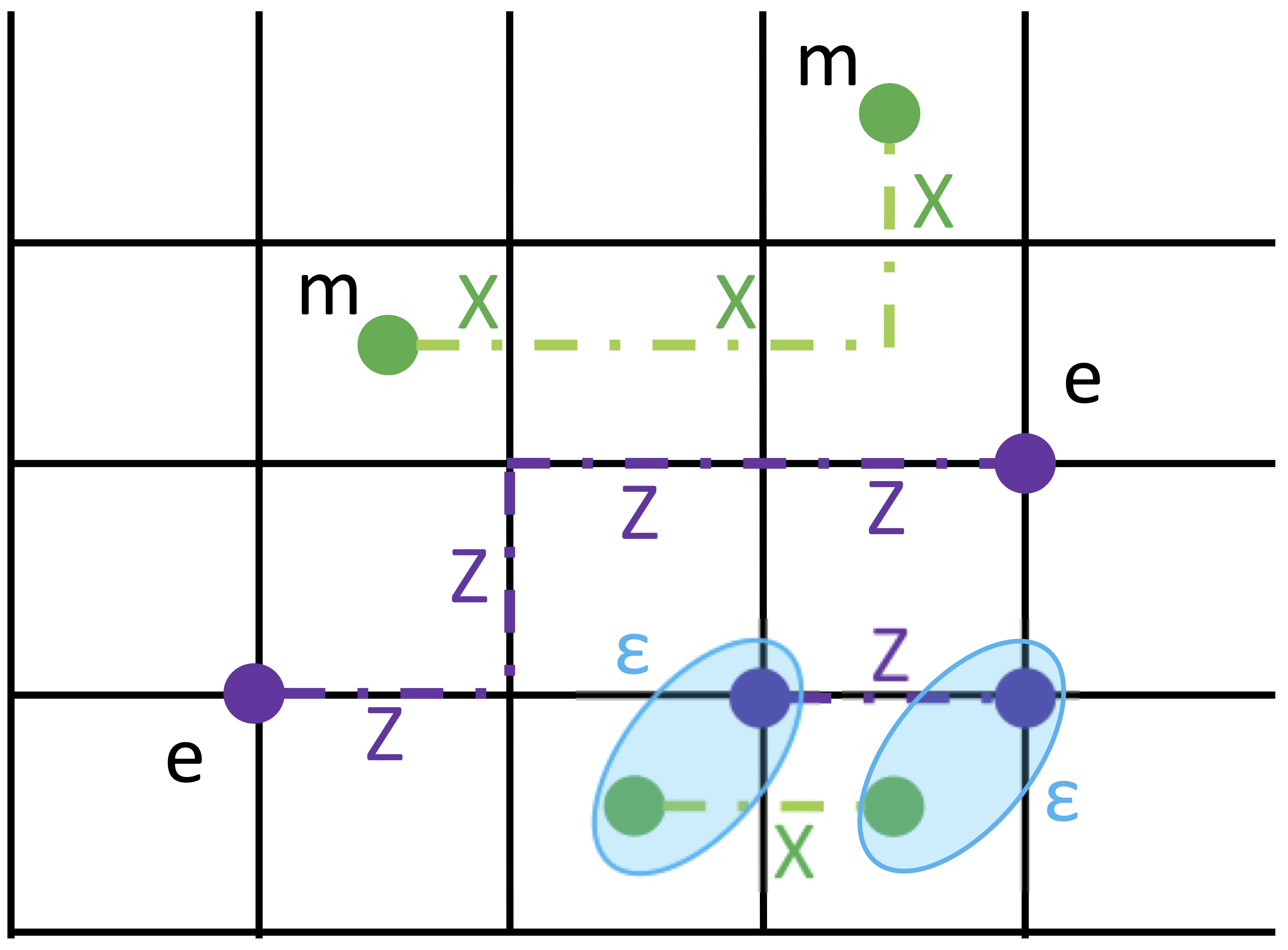
Fig. 6: Three types of quasiparticle excitations (anyons) in the toric code.

We can create a pair of quasiparticles excitations by applying string operators. String operators consist of product of Pauli \(X\) or \(Z\) operators applied to the qubits (see Fig. 6). A curious fact⁷ is that the total energy cost for the excitations created is dependent only on the number of excitations and not on a particular type of a string operator used e.g., both applying a single Pauli \(X\) operator costs the same amount of energy as applying (open) string of Pauli \(X\) operators of any other length⁸.

Fact 2: Excitations in the toric code (anyons) are always created in pairs by applying Pauli strings.

Single excitations

So far we have discussed how to create a pair of excitations. Is it possible to create a single, isolated, excitation by applying Pauli strings? Short answer: no. To see this, we first make the following observation \begin{equation} \prod_{\textrm{all} \ \ v} A_v = \mathbb{1} \ \ \ \prod_{\textrm{all} \ \ p} B_p = \mathbb{1} \end{equation} for the toric code defined on periodic boundary conditions (on torus) - as described in the previous sections⁹.

Exercise: Convince yourself (in drawing) that this observation is true.

Equipped with the observation above it is quite easy to show why the creation of single (or more generally any odd number of) excitations is impossible: this would yield the product of vertex/plaquette operator eigenvalues to be \(-1\) and to violate the condition in the above equation which holds throughout.

Loop excitations and error correction

Okay, so summarizing what we have arrived at so far: we cannot create single excitations by applying Pauli strings but we can easily create pairs of excitations. Given the “loopy” nature of the ground state we discovered in the first section we naturally ask: does anything interesting happen if the excitations form closed loops? Absolutely: it turns out that creating a topologically trivial closed loop of excitations is equivalent to creating no excitations at all. This is a really curious fact, so let me state it again in a different way: starting from a ground state we can create a set of excitations, pair them up (thus creating closed excitations loops) and get the ground state again! The physical intuition behind it is simple: since the ground states correspond to equal amplitude sum of closed loop configurations, the action of the closed loop string simply reorders the terms within the sum without changing the overall result! This “completing the loop” trick is one of the reasons why the toric code is useful for quantum error correction: if we say that the excitations were created by some unwanted “errors” in the form of Pauli strings then these errors might be annihilated by applying more Pauli strings and completing the loops.

Fact 3: Applying Pauli strings forming closed loops is equivalent to applying no string operators at all.

Anyons and their statistics

We found that the excitations of the toric code are “particle-like” and indistinguishable. Let’s try to understand what are the implications of this. In undergraduate quantum mechanics, we were taught that indistinguishable particles divide into two broad classes: bosons and fermions. Those differ by a sign acquired by the wavefunction under exchanging them (i.e. they pick up an extra \(\theta=0\) or \(\theta=\pi\) phase). What is interesting in (effectively) 2D systems is that sometimes those particle-like excitations can acquire any phase \(\theta \in [0,2 \pi )\) under exchange (hence those excitations are known as anyons). This idea (and the funny name for such particles) traces back to works of Frank Wilczek and colleagues in 1980s [Wilczek (1982)].

Now back to the toric code: can we classify its excitations by looking through the lens of exchange statistics? Yes, we say that there are three types of anyons in the toric code: \(e\) anyon (single vertex excitation), \(m\) anyon (single plaquette excitation) and \(\epsilon\) anyon (or a dyon) consisting of vertex and plaquette excitations bound together. \(e\) and \(m\) anyons in the toric code have abelian bosonic statistics i.e. the many-body state is invariant under exchanging two identical \(e\) and \(m\) anyons¹⁰.

It turns out that \(\epsilon\) anyons are fermions. To see this we need to first show that braiding the \(e\) particle around \(m\) particle (and vice-versa) accumulates \(-1\) phase. In other words we want to prove that \(\vert \psi_{final} \rangle = - \vert \psi_{init} \rangle\). The action of moving \(e\) around \(m\) might be written as \(\vert \psi_{final} \rangle = \prod_{j \in \textrm{loop}} Z_j \vert \psi_{init} \rangle\) and corresponds pictorially to the Fig. 7 below.

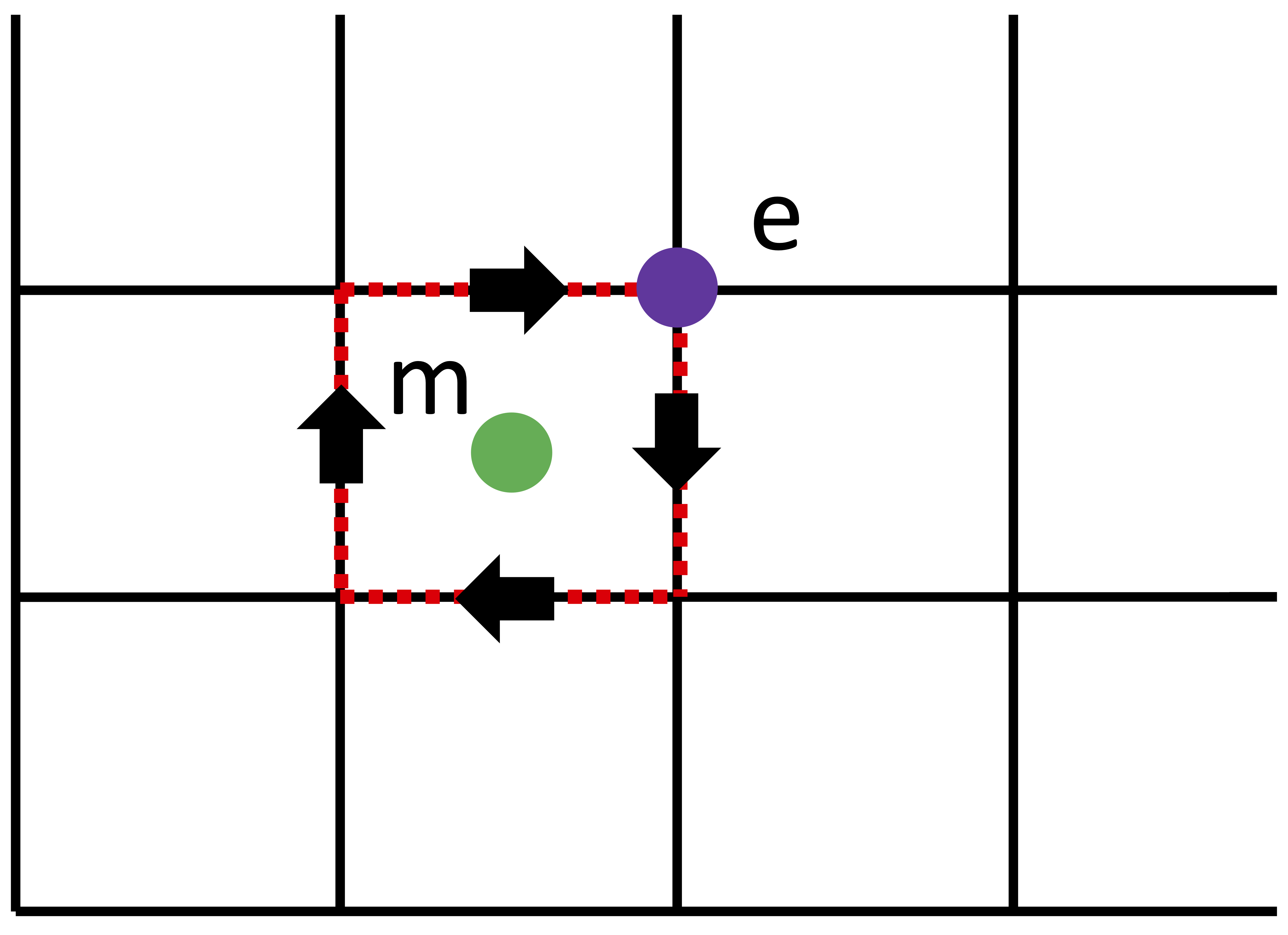
Fig. 7: Braiding \(e\) particle around \(m\) particle.

Noting that the product of the plaquette stabilizers enclosed by the loop is equal to \(-1\) (there is a single \(m\) excitation present inside the loop) i.e. \(\prod_{p \ \textrm{enclosed}} B_p \vert \psi_{init} \rangle = - \vert \psi_{init} \rangle\), and using the result of the exercise below we show what is intended.

Exercise: Show that \(\prod_j Z_{j \in \textrm{loop}} \vert \psi_{init} \rangle = \prod_{p \ \textrm{enclosed}} B_p \vert \psi_{init} \rangle\) Hint

Let’s pause here for a second and properly appreciate the above result. Note that the argument is true regardless of how far the \(e\) and \(m\) particles are: it means that \(e\) senses the presence of \(m\), even if they are separated very far away i.e. we are witnessing “spooky actions at a distance”¹¹ which demonstrate “long-range” structure of the entanglement (a topic which we will explore further in other blogposts!).

Okay, so braiding \(e\) around \(m\) accumulates \(-1\) phase for the state. Now, I claim that the proof of fermionic statistics of \(\epsilon\) particle follows from the Fig. 8 below [Kitaev&Laumann (2010) p. 15]:

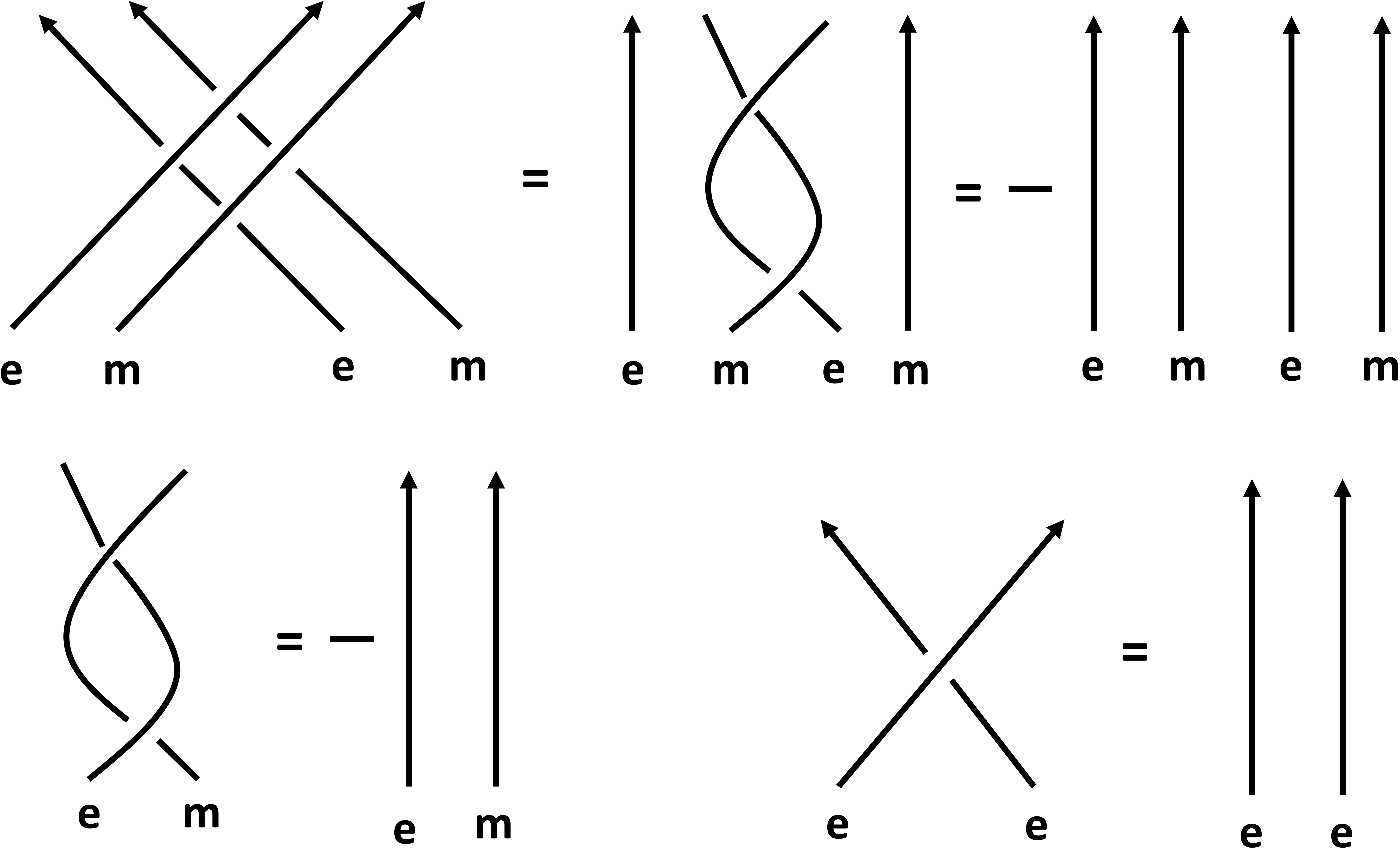
Fig. 8: Wordline braiding diagrams for the \(\epsilon\) particle consisting of an \(e\) and \(m\) bound together.

Okay, I understand that initially it might seem that there is a lot to unpack here, but in fact everything is plain and simple. Lines in Fig. 8 correspond to the \((2+1)-D\) worldlines of the anyons. Wordlines are nothing else than space-time graph¹² of the particle motion with time going up on the image and particles moving around each other in space (horizontal direction). We first draw the diagram corresponding to taking the \(e\) particle around \(m\) particle (considered above). Next, we utilize identities found before (bottom row) to simplify each of the crossings in the top row: picking up a \(-1\) factor for braiding \(e\) around \(m\) translates into the fermionic statistics of \(\epsilon\) particle!¹³ Although, all anyons in the toric code are still bosonic/fermionic, generalizations of the toric code (briefly described in the [FAQ]) that contain more exotic excitations.

Fact 4: Three types of (anyonic) excitations correspond to vertex, plaquette and “dyonic” violations and these have bosonic, bosonic and fermionic exchange statistics respectively.

Local indistinguishability

In the previous section, I stressed a few times that the excitation loops considered are the ones which are topologically trivial. What if we considered e.g., Pauli \(X\) strings which were making topologically non-trivial loops (e.g., ones corresponding to \(C_1, C_2 \ \textrm{or} \ C_3\) in Fig. 3)? Note that such non-trivial loops are automatically non-local since they need to traverse through the “whole system” (i.e. its size is at least \(L\), corresponding to the linear system size).

Let us take a ground state of the toric code, say the one consisting of topologically trivial loops. What happens if we now apply to it a topologically non-trivial Pauli string loop, say \(C_2\)? Linearity allows us to apply the topologically non-trivial string to each of the components in the closed-loop superposition: therefore now all of the terms within the superposition belong to the \(C_2\) equivalence class and the resulting state is thus another ground state \(\vert \psi_2 \rangle\) (as shown in Fig. 5). Applying the same argument to the other ground states we immediately notice the following

Fact 5: Ground states are locally indistinguishable i.e. may be mapped onto each other only by using non-local operators.

We might restate the above result in the following way: if an operator \(M\) is local (i.e. does not involve operators going through the “whole system”) then we have \(\langle \psi_i \vert M \vert \psi_j \rangle = C_M \delta_{ij}\) where \(C_M\) is a constant only dependent on \(M\). The shortest minimal distance of the non-local operator support is \(L\), which in error correction is known as a code distance (roughly speaking: the minimal length of an undetectable error).

Interestingly, local indistinguishability is one of the key components for a system to possess topological order i.e. loosely speaking to exhibit topology-dependent ground state degeneracy¹⁴ which cannot be removed¹⁵ by any local, sufficiently weak perturbation of the Hamiltonian [Zeng et al. (2015) p. 166]. In the case of the toric code, we indeed see the 4-fold ground state degeneracy which purely depends on the topology of the space and using local indistinguishability it might be shown that its ground state degeneracy cannot be lifted by any local, sufficiently weak perturbations [Bravyi et al. (2010)].

Conclusions

I hope I convinced you that the toric code is a model with some really cool properties. We have learnt what is the Hamiltonian describing the toric code, found its ground states (forming topologically equivalent closed loop configurations), shown how to create particle-like excitations (using Pauli strings), described their exchange statistics (which turned out to be bosonic for \(e\) and \(m\) and fermionic for \(\epsilon\) anyons), and discussed how toric code ground states are locally indistinguishable (paving the way to the concept of topological order). Huuh, that is a lot - well done going through all this stuff!

Obviously, there is still so much to say about the toric code! If this post still leaves you hungry for more stuff on the toric code (and beyond) see the FAQ section below with further reading suggestions, have a read of the complimentary post, and stay tuned for future blogposts on related topics!

FAQ

1. Can the toric code be defined only on a square lattice? No, in principle we can define toric code on any lattice. See e.g., [Simon (2020) Chp. 25.5].
2. Can the toric code be defined in the systems beyond 2D? Yes, in particular a 4D toric code is particularly interesting from the perspective of error correction since it might act as a self-correcting quantum memory¹⁶. For a gentle intro from a condensed matter-ish view on toric codes beyond 2D see e.g., [Savary&Balents (2016) p. 7].
3. Can the toric code be defined for systems other than qubits? Yes, for \(N\) level system we have \(Z_N\) toric code generalization; which we can further extend to more general groups in the so-called Kitaev double model (which can have non-Abelian anyons)! See e.g., [Simon (2020) Chp. 25.6 and Chp. 29]
4. Given the 4-body interaction term in the toric code Hamiltonian, can it be feasibly implemented in the lab? Yes, there are experimental demonstrations of a toric code in the lab (we will briefly discuss them in another blogpost!). If you particularly worry about the 4-body term specifically you might think of a toric code as the lowest order in perturbation theory description of the Kitaev Honeycomb model in the \(J_z \gg J_x,J_y\) regime: see e.g., [Kitaev (2006)].

Acknowledgements: I thank Arthur Pesah, Leo Lo and Quynh Nguyen for many fun discussions on toric code and beyond. I also thank Iria Wang and Shashvat Shukla for their helpful comments on the draft of this blogpost. Feel free to contact me at dkufel (at) g.harvard.edu if you have any questions or comments!

References

[Zeng et al. (2015)] Zeng, B., Chen, X., Zhou, D.L. and Wen, X.G., 2015. Quantum Information Meets Quantum Matter–From Quantum Entanglement to Topological Phase in Many-Body Systems. arXiv version.

[Simon (2020)] Simon, S.H., 2020. Topological Quantum: Lecture Notes and Proto-Book. Unpublished prototype. Online Open-Access.

[Wilczek (1982)] Wilczek, F., 1982. Quantum mechanics of fractional-spin particles. Physical review letters, 49(14), p.957. Online Open-Access

[Kitaev&Laumann (2010)] Kitaev, A. and Laumann, C., 2010. Topological phases and quantum computation. Exact methods in low-dimensional statistical physics and quantum computing, Lecture Notes of the Les Houches Summer School, (89), pp.101-125. arXiv version.

[Bravyi et al. (2010)] Bravyi, S., Hastings, M.B. and Michalakis, S., 2010. Topological quantum order: stability under local perturbations. Journal of mathematical physics, 51(9), p.093512 arXiv version.

[Kitaev (2006)] Kitaev, A., 2006. Anyons in an exactly solved model and beyond. Annals of Physics, 321(1), pp.2-111. arXiv version

[Savary&Balents (2016)] Savary, L. and Balents, L., 2016. Quantum spin liquids: a review. Reports on Progress in Physics, 80(1), p.016502. arXiv version

Hints to exercises

Hint: Whenever Pauli X and Z meet on the same site they anti-commute, otherwise (e.g., \([X \otimes \mathbb{1},\mathbb{1} \otimes Z]\) they commute.

Solution

Solution: First note that each vertex (plaquette) operator commutes with all other vertex (plaquette) operators (since all involve purely Pauli X (or Pauli Z) operators). Next, if plaquette operator and vertex operator do not touch one another they trivially commute (see hint). Finally even if we take plaquette operator touching vertex operator nearby, they will intersect on exactly two edges. On each edge Pauli operators anti-commute so their product will commute.

Hint: Think in spirit of the discrete version of Stokes’ theorem. Why should it apply here?

Solution

Solution: Consider a single plaquette. The product of \(Z\) operators around the plaquette corresponds simply to the \(B_p\) operator. Now take two plaquettes sharing an edge. The product of \(Z\) operators around these two plaquettes corresponds to a product of two \(B_p\) operators (this applies \(Z\) operator to the shared edge twice and thus is equivalent to applying no operator at all - exactly as required). You can now iterate this process to cover any set of connected plaquettes thus proving the desired statement.

1. If it does not immediately become clear why see this animation. ↩︎

2. Note that some people (see e.g., [Zeng et al. (2015)] or the complimentary blogpost) define \(A_v\) operators as products of Pauli \(Z\) operators; and \(B_p\) operators as products of Pauli \(X\) - this is just the matter of convention and does not change the physics in any essential way (since it corresponds to simply swapping \(X\)’s with \(Z\)’s i.e. a change of basis by conjugating all qubits with the Hadamard gate). ↩︎

3. If “topological inequivalence” does not ring a bell: loosely speaking we might say that two loops are “topologically inequivalent” if they cannot be smoothly deformed into one another. “Smoothly deforming” means that cutting/glueing and removing holes are not allowed. Roughly speaking, in topology we are concerned with the global properties of an object disregarding some local geometric details. For a high-level idea see a classic problem due to Euler. For a more proper introduction in the quantum error correction context check Arthur Pesah’s blogpost or those lecture notes. ↩︎

4. This language comes from quantum error correction. It means that the Hamiltonian is comprised of the terms which are stabilizers of an associated stabilizer quantum error code. To get a better feeling of what stabilizers are in the error correction formalism check out e.g., this blogpost. ↩︎

5. Just to recap: ground state at this stage just being a generic linear combination of closed loop configurations as described before. ↩︎

6. If it is not immediately clear think about associating to each point in the primal and dual lattice the eigenvalue of the corresponding vertex/plaquette operator. The ground state would simply correspond to all \(+1\) eigenvalues. Consequently regardless of where we create excitations to it - they will correspond to \(-1\) eigenvalue particle-like “peaks” in an otherwise uniform energy density background. ↩︎

7. There is quite a deep reason behind this, which we will explore more in the future blogpost. ↩︎

8. One might also create closed Pauli strings (i.e. those forming topologically trivial or non-trivial loops). Those, as we will discuss in sections on local indistinguishability and loop excitations cost no energy at all! ↩︎

9. This observation allows us to prove the 4-fold ground state degeneracy in an alternative way to the one described in the first section. The main idea is as follows: eigenvalues of each of the vertex/plaquette operators can be \(+1\) or \(-1\) (they are formed of Pauli operators which are both unitary and Hermitian); this means that there are \(2^N\) possible states. The conditions \(\prod_{\textrm{all} \ \ v} A_v = \mathbb{1} \ \ \ \prod_{\textrm{all} \ \ p} B_p = \mathbb{1}\), however, imply that two of these operators will not be independent: effectively we have \(2^{N-2}\) independent quantum numbers. This means that the ground state degeneracy will be \(2^N/2^{N-2}=4\). ↩︎

10. One way of showing this is to show that the “twist factor” in a topological quantum theory [Simon (2020) Chp. 26.2] is +1 (moving \(e\) (or \(m\)) particle involves only applying \(X\) (or \(Z\)) operators which all commute with each other). ↩︎

11. If the context is unfamiliar see this. ↩︎

12. Or in our case more of a 1D spatial projection of the 2D trajectory of the particle defined on a 2D toric code! ↩︎

13. In case this explanation was unclear or too quick: an alternative way of seeing this is the following. Imagine two \(e\) anyons connected by a Pauli \(X\) string. We can make them behave as an \(\epsilon\) anyon by attaching to each \(e\) anyon an \(m\) particle together with a long string (which connects to a copy of an \(m\) particles located at infinity - remember, we have shown that anyons always come in pairs!). Now exchanging two \(\epsilon\) particles would correspond to e.g., dragging one of the \(e\) particles (together with an \(m\) anyon and its string!) on a semicircle while the other along the shortest line connecting original positions of two anyons. One can see that at some point in this process, the Pauli \(X\) string attached to one of the \(m\) anyon will necessarily cross the Pauli string \(Z\) used to move \(e\) anyon - and since those anti-commute, such exchange will yield an extra minus sign! If this explanation does not help either: see e.g., [Simon (2020) Chp. 2 and Chp. 26.2]. ↩︎

14. Such degeneracy, curiously comes without breaking any underlying symmetry of the Hamiltonian. If this is not surprising I would encourage you to study the symmetry-breaking paradigm due to Landau. The point of the topological order is precisely to ‘disavow Landau’ as John Preskill would say (at least while disregarding generalization of the Landau’s paradigm to so-called “higher-form” symmetries). ↩︎

15. This in principle should be considered in the thermodynamic limit (infinite number of qubits), see [Bravyi et al. (2010)] p. 8. ↩︎

16. The main idea is as follows: loosely speaking, for quantum error correction, the longer the error string the larger chance that it corresponds to an uncorrectable error. As described before, the energy cost paid for the pair of excitations of any length is the same; for self-correcting memory (for storing quantum information) we want to retain non-locality of information encoding but yet penalize for longer excitation strings. It turns out that due to their dimensionality, 3D and 4D toric code energetically penalize long excitations one of the two or both types of Pauli errors respectively. ↩︎